
Trill Science Ministry| Chasers of the Lost Data
Team Updates
S
Sarah Price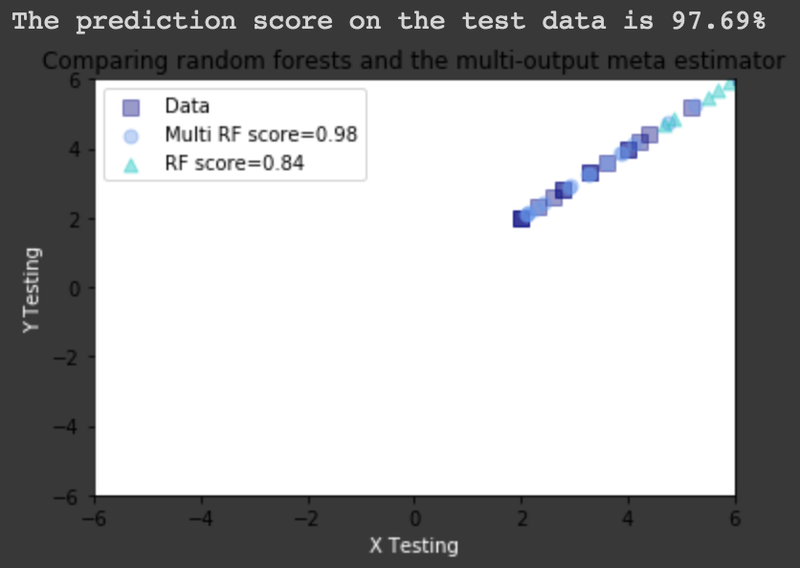
ML Testing output
Doing some neat visualization for our Chasers of the lost ark
This file contains hidden or bidirectional Unicode text that may be interpreted or compiled differently than what appears below. To review, open the file in an editor that reveals hidden Unicode characters. Learn more about bidirectional Unicode characters
| # -*- coding: utf-8 -*- | |
| """TrillApp.ipynb | |
| Automatically generated by Colaboratory. | |
| Original file is located at | |
| https://colab.research.google.com/drive/1b0qU_SkDafVEvhYmLhRgYzO_B-cu3KwQ | |
| """ | |
| # Tasks! | |
| ## Look at the Data | |
| ## Graph some portion of it | |
| ## Decide what portions we want to predict | |
| ## Research what kinds prediction options we have. | |
| ## Pick two and see which one seems to have the best results immediately. | |
| ## Work on perfecting the solution | |
| src='https://data.nasa.gov/api/views/mc52-syum/rows.csv?accessType=DOWNLOAD' | |
| # Space Apps Challenge | |
| # Lost Data Chasers | |
| importpandasaspd | |
| importnumpyasnp | |
| # Read data into variable | |
| data=pd.read_csv(src) | |
| cleanData=data.dropna() | |
| print(data.columns) | |
| withpd.option_context('display.max_rows', None, 'display.max_columns', None): # more options can be specified also | |
| print(data) | |
| importrequests | |
| response=requests.get('https://ssd-api.jpl.nasa.gov/fireball.api?limit=2000&vel-comp=true') | |
| # from pandas.io.json import json_normalize | |
| # print(response.json()['data']) | |
| x=response.json() | |
| print(x.keys()) | |
| df=pd.DataFrame(x['data'], dtype=float) | |
| # df = pd.io.json.json_normalize(response.json) | |
| # df = pd.read_json() | |
| df.columns=x['fields'] | |
| # print(df) | |
| print(x['fields']) | |
| print(x['count']) | |
| print(x['signature']) | |
| withpd.option_context('display.max_rows', None, 'display.max_columns', None): | |
| print(df[:40]) #.dropna() | |
| df_na_free=df.dropna() | |
| print(df_na_free[:6]['vel'].to_list()) | |
| df_na_free['vel'] =pd.to_numeric(df_na_free['vel']) | |
| df_na_free['impact-e'] =pd.to_numeric(df_na_free['impact-e']) | |
| df_na_free.plot(x='impact-e',y='vel',kind='scatter') | |
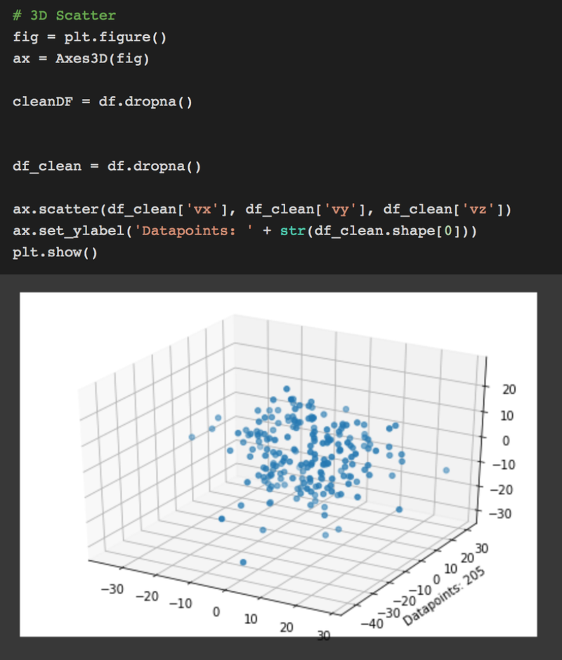
| # 3D Scatter | |
| importmatplotlib.pyplotasplt | |
| frommpl_toolkits.mplot3dimportAxes3D | |
| fig=plt.figure() | |
| ax=Axes3D(fig) | |
| cleanDF=df.dropna() | |
| df_clean=df.dropna() | |
| ax.scatter(df_clean['vx'], df_clean['vy'], df_clean['vz']) | |
| ax.set_ylabel('Datapoints: '+str(df_clean.shape[0])) | |
| plt.show() | |
| df_print_all=df.dropna() | |
| print(df_na_free[:6]['vel'].to_list()) | |
| df_na_free.plot(x='impact-e',y='vel',kind='scatter') | |
| """# Machine Learning""" | |
| fromsklearn.datasetsimportmake_regression | |
| fromsklearn.linear_modelimportLinearRegression | |
| temp=df.copy() | |
| temp.drop(['date'], axis=1, inplace=True) | |
| temp.loc[df['lat-dir'] =='S', 'lat-dir'] =-1 | |
| temp.loc[df['lat-dir'] =='N', 'lat-dir'] =1 | |
| temp.loc[df['lon-dir'] =='E', 'lon-dir'] =1 | |
| temp.loc[df['lon-dir'] =='W', 'lon-dir'] =-1 | |
| #X,y = make_regression(n_samples=len(df.dropna()), n_features=9, n_informative=3, n_targets=9, tail_strength=0.5, noise=0.02, shuffle=False, coef=False, random_state=0) | |
| X=temp | |
| y=temp | |
| icols=temp.columns | |
| jcols=icols | |
| ML=pd.concat([pd.DataFrame(X, columns=icols), pd.DataFrame(y, columns=jcols)], axis=1) | |
| ML.head() | |
| fromsklearn.ensembleimportRandomForestRegressor | |
| fromsklearn.multioutputimportMultiOutputRegressor | |
| fromsklearn.model_selectionimporttrain_test_split | |
| importmatplotlib.pyplotasplt | |
| df_notnans=ML.dropna() | |
| fromwarningsimportsimplefilter | |
| simplefilter(action='ignore', category=FutureWarning) | |
| X_train, X_test, y_train, y_test=train_test_split(df_notnans[icols], df_notnans[jcols], train_size=0.81, random_state=4) | |
| max_depth=30 | |
| regr_multirf=MultiOutputRegressor(RandomForestRegressor(max_depth=max_depth, | |
| random_state=0)) | |
| regr_multirf.fit(X_train, y_train) | |
| regr_rf=RandomForestRegressor(max_depth=max_depth, random_state=2) | |
| regr_rf.fit(X_train, y_train) | |
| # Predict on new data | |
| y_multirf=regr_multirf.predict(X_test) | |
| y_rf=regr_rf.predict(X_test) | |
| # Check the prediction score | |
| scores=regr_multirf.score(X_test, y_test) | |
| print("The prediction score on the test data is {:.2f}%".format(scores*100)) | |
| plt.figure() | |
| s=50 | |
| a=0.4 | |
| plt.scatter(y_test.iloc[:, 0], y_test.iloc[:, 1], | |
| c="navy", s=s, marker="s", alpha=a, label="Data") | |
| plt.scatter(y_multirf[:, 0], y_multirf[:, 1], | |
| c="cornflowerblue", s=s, alpha=a, | |
| label="Multi RF score=%.2f"%regr_multirf.score(X_test, y_test)) | |
| plt.scatter(y_rf[:, 0], y_rf[:, 1], | |
| c="c", s=s, marker="^", alpha=a, | |
| label="RF score=%.2f"%regr_rf.score(X_test, y_test)) | |
| plt.xlim([-6, 6]) | |
| plt.ylim([-6, 6]) | |
| plt.xlabel("X Testing", color='white') | |
| plt.ylabel("Y Testing", color='white') | |
| plt.title("Comparing random forests and the multi-output meta estimator") | |
| plt.legend() | |
| plt.show() |