The Mars Society Chile - Space Apps Challenge

The Mars Society Chile| Spot That Fire V2.0

Team Updates

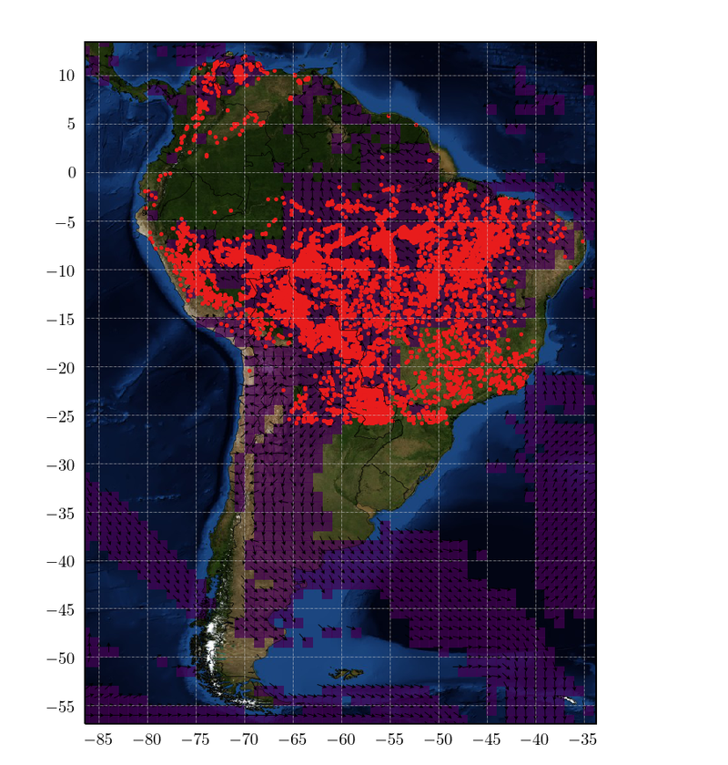
The figure shows the zones with a higher risk of fires (purple areas) and active wildfire (red dots) on August 4, 2019, between 12:00 and 18:00 UTC.

Jorge Gacitúa Gutiérrez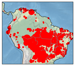

Figure for August 20, 2019 wildfire risk at Amazon Forest and countries from South America, based on data from https://firms.modaps.eosdis.nasa.gov both MODIS Terra/Aqua and VIIRS.

Pamela Pizarro

	# -- coding: utf-8 --
	importnumpyasnp
	fromnetCDF4importDataset
	importpandasaspd

	fromdatetimeimportdatetimeasdt
	fromdatetimeimporttimedelta

	importcartopy.io.shapereaderasshpreader
	fromcartopy.featureimportShapelyFeature

	importmatplotlib.pyplotasplt
	frommatplotlibimportrc
	frommatplotlibimportrcParams
	importmatplotlib.axesasmaxes
	importmatplotlib.tickerasmticker
	importcartopy.crsasccrs
	frommpl_toolkits.axes_grid1importmake_axes_locatable
	importscipy.ndimage
	importmatplotlib.imageasmpimg


	defRead_gfs(file_in):
	dataset=Dataset(file_in)
	lat=dataset.variables['lat_0'][:] # vector de Latitudes
	lon=dataset.variables['lon_0'][:] # vector de Longitudes
	U=dataset.variables['UGRD_P0_L103_GLL0'][0,:,:] # matriz de viento zonal a 10 m [lat,lon]
	V=dataset.variables['VGRD_P0_L103_GLL0'][0,:,:] # matriz de viento meridional a 10 m [lat,lon]
	#z = dataset.variables['lv_HTGL7'][:]
	T=dataset.variables['TMP_P0_L103_GLL0'][0,:,:] -273.15# matriz de temperatura a 0 m [lat,lon]
	RH=dataset.variables['RH_P0_L103_GLL0'][:] # matriz de humedad relativa a 2 m [lat,lon]

	returnlat, lon, U, V, T, RH


	deffire_index(lat,lon, U, V, T, RH, spd_val, T_val, RH_val):
	spd=np.sqrt(UU+VV)
	a=np.ones(np.shape(spd))
	#RH_data = np.ma.masked_where(RH >= RH_val,a)
	#spd_data = np.ma.masked_where(spd <= spd_val,a)
	#T_data = np.ma.masked_where(T <= T_val,a)

	fire_data=np.ma.masked_where(np.logical_and(T<=T_val, np.logical_and(spd<=spd_val,RH>=RH_val)),a)
	U_data=np.ma.masked_where(np.logical_and(T<=T_val, np.logical_and(spd<=spd_val,RH>=RH_val)),U)
	V_data=np.ma.masked_where(np.logical_and(T<=T_val, np.logical_and(spd<=spd_val,RH>=RH_val)),V)
	spd_data=np.ma.masked_where(np.logical_and(T<=T_val, np.logical_and(spd<=spd_val,RH>=RH_val)),spd)
	lon_data=np.ma.masked_where(np.logical_and(T<=T_val, np.logical_and(spd<=spd_val,RH>=RH_val)),lon)
	lat_data=np.ma.masked_where(np.logical_and(T<=T_val, np.logical_and(spd<=spd_val,RH>=RH_val)),lat)


	returnfire_data, U_data, V_data, spd_data, lon_data, lat_data#RH_data+spd_data+T_data


	defplot_fire_index(lat,lon, U, V, T, RH,fire_spots,h):
	'''
	La funcion para graficar el mapa y los datos entregados.
	'''

	############################################################################
	###################### Lectura de focos de incendios #######################
	############################################################################
	datafirem6=pd.read_csv(fire_spots)

	lat_frp=datafirem6['latitude'].values
	lon_frp=datafirem6['longitude'].values
	frp=datafirem6['frp'].values
	time_frp=datafirem6['acq_time'].values
	hour_frp=np.floor(time_frp/100)
	mn=np.median(frp)

	idx_median, =np.where(frp>mn) # aca se indican los indices de los valores que cumplen la condicion

	fire_f=frp[idx_median]
	lat_ff=lat_frp[idx_median]
	lon_ff=lon_frp[idx_median]
	hour_ff=hour_frp[idx_median]
	##### ahora se seleccionnan solo las 6 horas anteriores a la indicada
	idx_hour, =np.where(np.logical_and(hour_ff>=h-6,hour_ff<=h))
	fire=fire_f[idx_hour]
	lat_f=lat_ff[idx_hour]
	lon_f=lon_ff[idx_hour]


	########################### datos meteorologicos ###########################

	x,y=np.meshgrid(lon,lat)
	fire_data, U_data, V_data, SPD_data, lon_data, lat_data=fire_index(y,x, U, V, T, RH, 8.3, 30, 30)

	############################################################################
	############################# Grafico de mapa ##############################
	############################################################################

	extent= [-86.4844, -33.7500, -56.8828, 13.4297]
	lon0=0.5*(extent[0] +extent[1])
	proj=ccrs.PlateCarree()
	width=6
	height=width*(860/800)

	############################ plot Fire index #############################

	plt.rc('text', usetex=True)
	plt.rc('font', family='serif')

	fig=plt.figure(figsize=(width,height), dpi=150)
	axr=fig.add_subplot(1, 1, 1, projection=proj)

	shpfilename=shpreader.natural_earth(resolution='10m',
	category='cultural',
	name='admin_0_countries')
	axr.set_extent(extent,crs=proj)

	img=mpimg.imread('BlueMarble.jpg')
	plt.imshow(img,extent=[-180, 180, -90, 90])

	gl=axr.gridlines(crs=proj, draw_labels=True, linewidth=0.25,
	color='lightgray', linestyle='-.')
	gl.xlabels_top=False
	gl.ylabels_right=False
	gl.xlocator=mticker.FixedLocator(np.arange(-90, -25, 5))
	gl.ylocator=mticker.FixedLocator(np.arange(-60, 20, 5))

	Data_map=axr.pcolor(lon, lat, fire_data, transform=proj, alpha=0.7)
	axr.quiver(lon_data, lat_data, U_data/SPD_data,V_data/SPD_data,pivot='middle', units='dots',
	scale_units='dots', scale=0.08, headwidth=6,
	headlength=6, width=0.9,transform=proj)
	axr.scatter(lon_f, lat_f, s=2,c='#e81c1c',transform=proj) # aca se grafican los focos

	borde_feature=ShapelyFeature(shpreader.Reader(shpfilename).geometries(),
	proj, edgecolor='k', linewidth=0.2)
	axr.add_feature(borde_feature, facecolor='none')



	#axr.set_title('Fuego Fuego Fire Fire')

	plt.subplots_adjust(top=0.945,bottom=0.054,left=0.025,right=0.91,hspace=0.2,wspace=0.2)
	plt.show()


	if__name__=="__main__":
	file_in='fnl_20190804_18_00.grib2.nc'
	lat, lon, U, V, T, RH=Read_gfs(file_in)
	plot_fire_index(lat,lon, U, V, T, RH,"fire_nrt_M6_81341.csv",18)

view raw Read_GFS.py hosted with ❤ by GitHub

Jorge Gacitúa Gutiérrez

The figure below shows fire danger during amazon wildfire, on august 20, 2019.

Pamela Pizarro

figure using firm data, analizing fire danger

Pamela Pizarro