
Full_of_Hot_Air| Surface-to-Air (Quality) Mission
Team Updates
As a resident in California, constantly we are seeing fire, traffic, a large amount of moving-in population and other factors that can influence the air quality here in Los Angeles. We want to showcase whether these factors can remarkably affect the air quality and AOD3 volume which is a main harmful particle. We also want to know if air quality in recent years is better or worse than 3 or 5 years ago and predict future air quality.
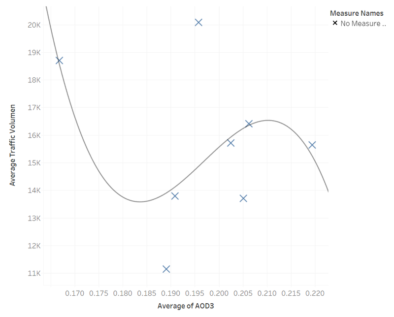
We collected data from provided data resource which contains the date, location, and average AOD3 volume. We find other resources, like population density by zip code in Los Angeles in 2010 and total traffic volume from 2003 to 2010. We think that daily traffic volume is hard to parse from 2010 to 2019, thus we omit it and only compare the traffic volume with the AOD3 from 2003 to 2010.
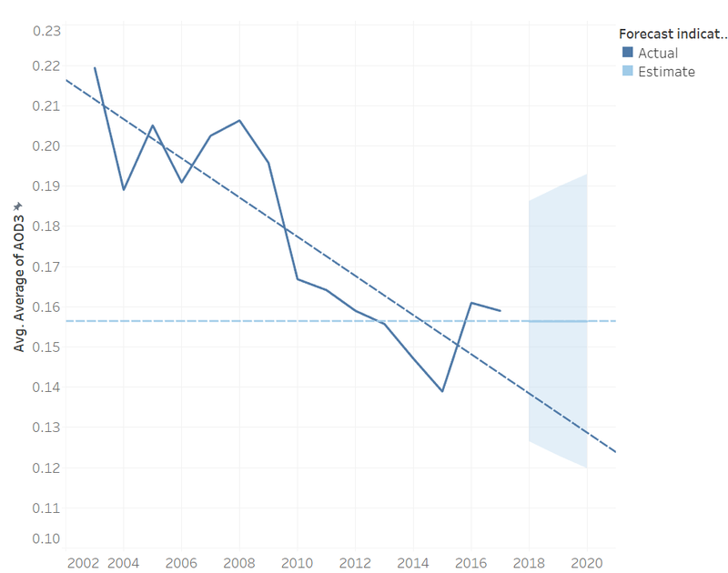
We spent two-quarter of the time to clean the data and using multiple linear regression model, decision tree model to predict the AOD3 by year and month, respectively. We found the r square(a statistic term) is around 0.7, showing there is a strong relationship between year and AOD3. Finally, we used a visualized tool to illustrate the analysis.
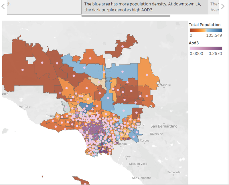
It is found that the air quality is worse in the area of high population density compared to the suburban area. There is no significant relationship between AOD3 and total traffic volume from 2003 to 2010. The air quality is getting better than previous years.
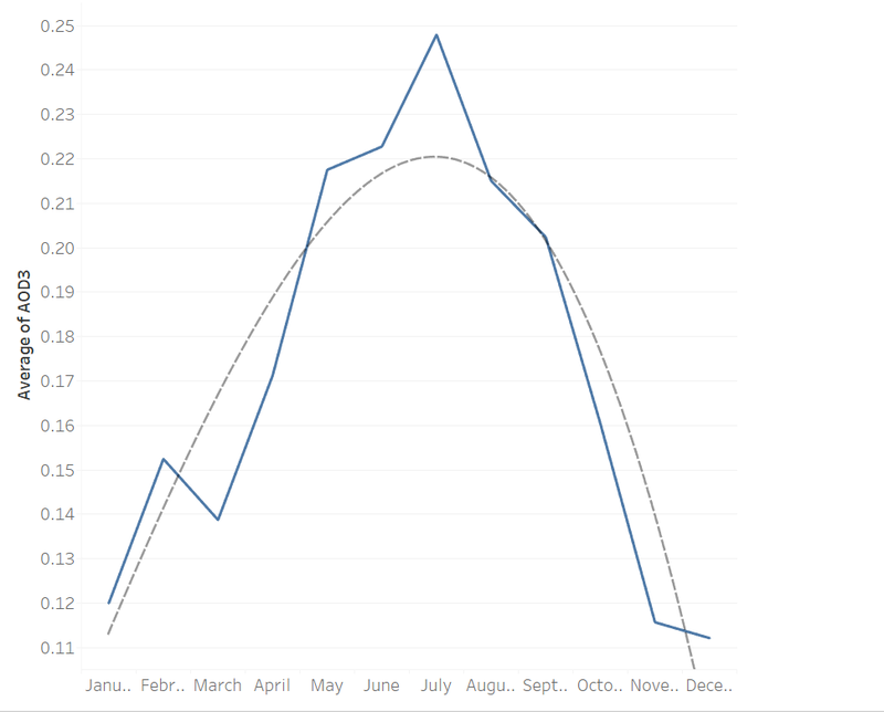
| #visualize AOD3 by month | |
| import pandas as pd | |
| raw_data=pd.read_csv('AOD_Combined.csv') | |
| df= pd.DataFrame(raw_data) | |
| df=df.sort_values(by=['Year','Month','Day']) | |
| df_group=df.groupby('Month').mean() | |
| aver_AOD3=df_group.iloc[: , 5] | |
| y=aver_AOD3 | |
| x=[1,2,3,4,5,6,7,8,9,10,11,12] | |
| import matplotlib.pyplot as plt | |
| scatter=plt.scatter(x,y,alpha=0.5) | |
| #Visualize AOD3 by year | |
| df_group2=df('Year').mean() | |
| aver_AOD3_2=df_group2.iloc[:,5] | |
| y2=aver_AOD3_2 | |
| x2=[2000,2001,2002,2003,2004,2005,2006,2007,2008,2009,2010,2011,2012,2013,2014,2015,2016,2017,2018,2019] | |
| import matplotlib.pyplot as plt | |
| scatter=plt.scatter(x2,y2,alpha=0.5, color='red') | |
| # R Squared detemination | |
| x_R= df.iloc[: , 0].values | |
| y_R= df.iloc[:,6].values | |
| results = {} | |
| import numpy | |
| x1 = numpy.array(x_R) | |
| y1 = numpy.array(y_R) | |
| coeffs = numpy.polyfit(x1, y1, 1) | |
| results['polynomial'] = coeffs.tolist() | |
| yhat = p(x_R) | |
| ybar = numpy.sum(y1)/len(y1) | |
| ssreg = numpy.sum((yhat-ybar)**2) | |
| sstot = numpy.sum((y1 - ybar)**2) | |
| results['determination'] = ssreg / sstot | |
| # Multiple Linear Regression | |
| import numpy as np | |
| x_new=df.iloc[:,:3].values | |
| y_new=df.iloc[:,6].values | |
| from sklearn.model_selection import train_test_split | |
| X_train, X_test, y_train, y_test=train_test_split(x_new,y_new, test_size=0.2, random_state=0) | |
| from sklearn.linear_model import LinearRegression | |
| regressor=LinearRegression() | |
| regressor.fit(X_train, y_train) | |
| new_data_set={'Year':[2019,2019,2019,2019,2019,2019,2019,2019,2019,2019,2019,2019],'Month':[1,2,3,4,5,6,7,8,9,10,11,12],'Day':[22,22,22,22,22,22,22,22,22,22,22,22]} | |
| new_data=pd.DataFrame(new_data_set) | |
| pred=regressor.predict(new_data) | |
| raw_data1=pd.read_csv('AOD_Combined.csv') | |
| df1= pd.DataFrame(raw_data) | |
| df1=df.sort_values(by=['Year','Month','Day']) | |
| x_new1=df.iloc[:,1:3].values | |
| y_new1=df.iloc[:,6].values | |
| #using decision tree regression | |
| from sklearn.model_selection import train_test_split | |
| X_train3, X_test3, y_train3, y_test3=train_test_split(X_x,Y_y, test_size=0.25, random_state=0) | |
| X_train3= X_train3.reshape(-1, 1) | |
| y_train3= y_train3.reshape(-1, 1) | |
| X_test3 = X_test3.reshape(-1, 1) | |
| from sklearn import preprocessing | |
| from sklearn import utils | |
| lab_enc = preprocessing.LabelEncoder() | |
| encoded = lab_enc.fit_transform(X_train3) | |
| from sklearn import preprocessing | |
| lab_enc = preprocessing.LabelEncoder() | |
| encoded = lab_enc.fit_transform(X_test3) | |
| from sklearn.preprocessing import StandardScaler | |
| sc=StandardScaler() | |
| X_train3=sc.fit_transform(X_train3) | |
| X_test3=sc.transform(X_test3) | |
| from sklearn.svm import SVC | |
| classifier=SVC(kernel='linear',random_state=0) | |
| classifier.fit(X_train3.reshape(-1,1), y_train3) | |
| y_pred3=classifier.predict(X_test3) | |
| Y_pred3=classifier.predict(new_data) |